Multi-Scale DenseNet, a resource-aware CNN
ICLR 2018 - 3rd article
In this series, we explore the 2018 edition of the International Conference on Learning Representations. Oral papers are analyzed and commented in an accessible way.
This article is based on the paper Multi-Scale Dense Networks for resource efficient image classification by Gao Huang, Danlu Chen, Tianhong Li, Felix Wu, Laurens van der Maaten and Kilian Weinberger.
Introduction
Have a look at the two pictures below. It probably took you an unnoticeable amount of time to recognize a horse on the left, and a very noticeable amount of time (say one second) to recognize a horse on the right. Naturally, we would expect models to face similar difficulties in classification of those images. Intuitively, it feels like a simple CNN with a couple layers (e.g. AlexNet) would be more than enough to classify the first picture, while the last one shall require a much more complex model for correct classification, being in the tail of the “horse images” distribution (hence requiring a more precise approximation of this distribution by a neural network).
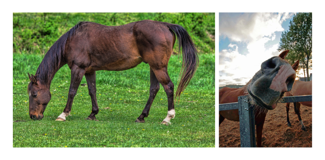
Using the same model to classify both pictures generally means that you have to choose beforehand, and once and for all (when you implement the model), between low resource consumption and high accuracy. In other words:
Computationally intensive models are needed to classify such tail examples correctly, but are wasteful when applied to canonical images such as the left one.
Now, generally speaking, we computer users don’t care, or at least this is not a question that we are used to ask. In the rare situations where we actually care about resource consumption (most of all about speed), we just define a minimum acceptable inference speed, pick the best performing model that satisfies this constraint, and that’s basically it. However, we phone users and (future) Internet of Things users are very much likely to care. From photo deblurring to real-time action recognition, computer vision will become ubiquitous in everyday devices, that run on much lower resources than modern computers. Moreover, lower computational cost means lower time energy consumption, which is highly desirable for ecological (and economical) reasons.
All in all, it feels frustrating not to recognize a horse on the right, so we use the winner of ImageNet 2017 (an ensemble of Squeeze-and-Excitation Networks); but it is ridiculous to waste 440 MB of parameters and 21 GFLOPs on recognizing a horse on the right while we probably only need 50 times less resources to do it (as a reference, Apple’s iPhone 4 had a processor power of about 3 GFLOP/s, so it would actually take 7 seconds at 100% CPU to process each image). We feel torn between both issues, and nobody likes feeling torn.
This begs the question: why do we choose between either wasting computational resources by applying an unnecessarily computationally expensive model to easy images, or making mistakes by using an efficient model that fails to recognize difficult images? Ideally, our systems should automatically use small networks when test images are easy or computational resources limited, and use big networks when test images are hard or computation is abundant.
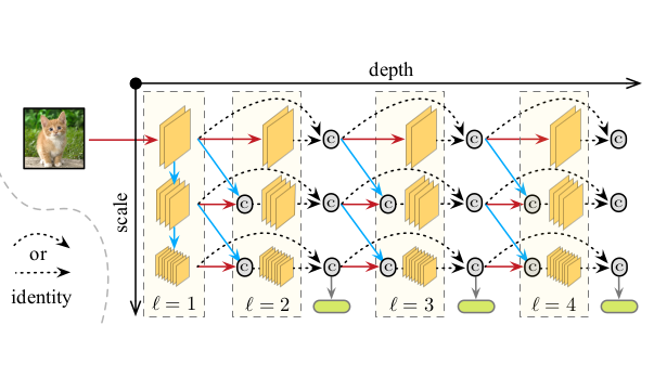
This is why the authors propose the Multi-Scale Dense Network model (architecture below), which we will explore, that enables adaptive resource allocation for image classification thanks to the introduction of early classifiers in a feed-forward CNN structure. This way, easy images can be instantly classified, and harder ones can use more computational resources. Let’s see how this works on real-world tasks.

Real-word tasks - classification on a (tight) budget
Let’s first define the situations where a resource-aware model is likely to be more useful than an off-the-shelf CNN. This will help us understand where and when exactly the new architecture helps. Computationally constrained tasks are numerous and diverse, and we will only focus on two major problems: anytime prediction, and budgeted batch classification.
Anytime prediction
In anytime prediction, the model can be forced to output a prediction, at any given point, possibly before the full computation is complete. Good performance levels are typically achieved by models that are able to give crude estimates very quickly, and refine them with time until the full model is run. For example, imagine an autonomous car equipped with a network to detect and handle obstacles on the road. You want your car to instantly detect and react to a pedestrian suddenly appearing in front of the car; there is no time to decide the precise distance at which it appears, whether it is an adult or a child, and at which speed it is going towards you. On the other hand, for distant and long-term obstacles, determining the precise distance between you and them enables better planning, smooth trajectories, better fuel management, etc.
In a formal way, we assume that test samples $x$ and budgets $B$ are drawn from a joint distribution $P(x, B)$. The model outputs a prediction $f(x)$ within the computational budget $B$, and incurs a loss $L(f(x), B)$. The goal in anytime prediction is to find a model that minimizes the expected loss of individual prediction within (hard) budget constraint:
[\min_f \ \mathbb{E}_{P(x, B)} [L(f(x)), B]]
Another example of anytime prediction is real-time video classification. You are filming a scene, and you want your phone to identify the various elements present in the video while filming. It is not unreasonable to ask for a refresh rate of 10 Hz, which means a prediction every 0.1 s, whatever the computational budget available on your phone at that time.
Budgeted batch classification
In budgeted batch classification, the model is granted a finite known computational budget to classify a set of examples, and can spend it freely across examples. Good performance levels are typically achieved by models that are able to quickly classify easy examples (left horse), in order to save some additional computation for harder examples (right horse). For example, imagine that you want to show your best friend all the pictures on your phone where both of you are present. Some pictures will be easily classified (you both clearly face the camera, no other people present), some will be much harder (you are in a crowd, disguised, wearing make-up or making funny faces). You don’t care much about that, and you only want your phone to give you a decent search result in less than 5 seconds.
Formally, we consider a set of examples $\mathcal{D}_ {test} = \{ x_1, …, x_M \}$ and a computational budget $B$ that is known in advance. The model spends $B$ as it pleases across examples, outputs a set of predictions $f(\mathcal{D}_ {test})$ and incurs loss $L(f(\mathcal{D}_{test}), B)$. The goal in budgeted batch classification is to find a model that minimizes the expected loss of batch prediction within (soft) budget constraint:
[\min_f \ \mathbb{E}{P(x)} [L(f(\mathcal{D}{test})), B]]
The problems with early classification
Let us think it through. The simplest, most natural answer to address both these situations is to use multiple networks with increasing capacity (e.g. multiply the number of layers by a constant factor from one model to the next one), and evaluate them sequentially at test time. In anytime prediction, you simply output the prediction of the last network evaluated; in batch budgeted classification, you stop the evaluation once classification with sufficient confidence level is reached. This is illustrated in the next figure:
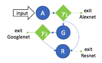
A “sequence of models” solution, featuring AlexNet (A), GoogLeNet (G) and ResNet (R). Green $\gamma$ blocks denote selection policies. The input is first evaluated by AlexNet, and the selection policy determines whether evaluation by more complex models is needed. (Source)
The problem with this approach is that, when the first network isn’t confident enough, we switch to the second network without re-using any feature previously computed: for complex examples, we completely waste the computational budget spent on the first networks. This is quite unsatisfying, and far from optimal.
Then the opposite solution comes in mind: instead of building multiple networks with one classifier each, not sharing any feature, we could build one network as a cascade of multiple (early) classifiers along depth, re-using previous features to build the more advanced predictions. This would look like the next figure:
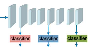
A simple “cascade of classifiers” solution on a standard CNN architecture. Early classification of easy examples yields substantial savings in computational budget, that can be spend on the hard examples. (Source)
Although this model doesn’t waste any feature, it leads to poor performance, for two distinct reasons:
- Early classifiers lack coarse-level, global features - only fine-scale, local features are available at early stages.
- Early classifiers interfere with later classifiers - early classifiers tend to optimize the early features for the short-term, conflicting with the long-term optimization of late classifiers, that achieve better performance.
These two issues will drive the design of MSDNet through the inclusion of two specific components, each addressing one issue.
Early classifiers vs. dense connections
Let us take a common CNN architecture, ResNet, and attach an intermediate classifier at a (more or less) early stage of the architecture. We then train both (final and intermediate) classifiers jointly (here on CIFAR-100), weighting their losses equally, and look at the accuracy of the final classifier. If there a noticeable difference in performance with the standard setting, the presence of the intermediate classifier is likely to have an influence on the construction of the features.
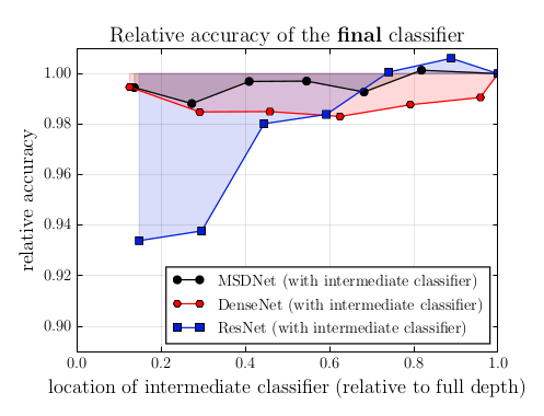
As is clear from the figure, ResNet performance generally suffers a lot from the introduction of an intermediate classifier, especially at very early stages.
We postulate that this accuracy degradation in the ResNet may be caused by the intermediate classifier influencing the early features to be optimized for the short-term and not for the final layers. This improves the accuracy of the intermediate classifier but collapses information required to generate high quality features in later layers.
This sounds like a reasonable and likely hypothesis. It would be interesting to visually examine the filters learned and the corresponding features for different locations of the intermediate classifier, providing us with some insights in this regard.
Solution/Mitigation: Dense connections
To mitigate this problem, the paper cites dense connections as an interesting line of work. Dense connections were introduced by our authors one year earlier in DenseNets, as a generalization of residual connections, the building blocks of ResNets. Remember what a residual connection looks like? A residual block is displayed in the next figure: the signal can bypass the layer thanks to an identity connection, and addition with the layer’s output.
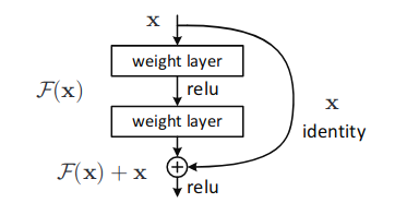 A residual block, the building foundation of ResNets. (Source)
Dense connections go one step further by connecting each layer directly with all previous layers (inside the same block). What’s more, instead of being summed, the previous features are concatenated to enable direct re-use. The resulting dense block is illustrated in the next figure:
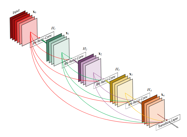 A dense block, the building foundation of DenseNets. At each stage, the features of all previous layers are concatenated to maximize information flow and allow layer bypassing as much as possible. (Source)
Now how will this help us? Compared to ResNets, DenseNets suffer much less from the introduction of intermediate classifiers at early levels (see the figure some blocks above). This is likely linked to the fact that the signal can bypass all layers, so that no layer results in a loss in information. Should an early layer get optimized for short-term classification, the original signal can still be recovered unperturbed by later layers. This greatly alleviates the influence between short-term and long-term optimization, and makes the final accuracy of DenseNets not too dependent on the location of the intermediate classifier, yielding a nice candidate to support early classifiers.
Coarse features vs. multiple scales
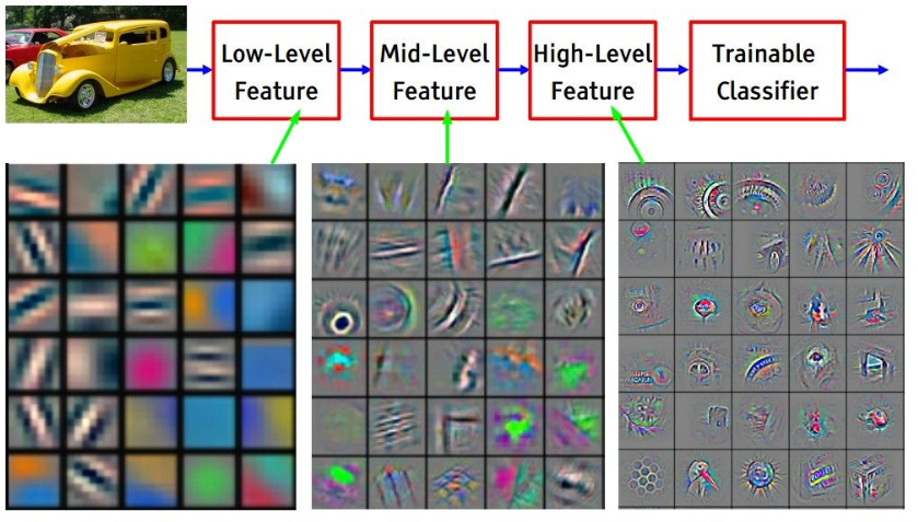
Visualization of the features learned by a convolutional network along its depth, using DeconvNet. Low-level features match local and simple patterns, while higher level features retain incresingly global and complex patterns. (Source)
You’ve probably seen this picture a couple times already, or one alike. This visualization of the features learned by the network along the depth was obtained thanks to a visualization DeconvNet. It supports the claim that first layers correspond to local, fine-scale features (the feature maps learned are close to the size of the original image), whereas deep layers correspond to global, coarse-scale features (the feature maps learned are much smaller than the original image, condensing global information such as “there is a dog in this region”).
Now this is a problem for early classifiers. Image classification is much harder when you only have access to local features, matching only simple patterns such as straight lines in different directions, or circles of different sizes. To confirm this intuition, let us consider again our previous experiment: take a ResNet, attach an intermediate classifier at different locations along the depth of the network, but this time examine how this location influences the accuracy of the intermediate classifier. If classification based on local, fine-scale features was as easy as classification based on global, coarse-scale features, the impact on accuracy should not be too noticeable (and, as a side note, we woudln’t need deep learning to begin with).
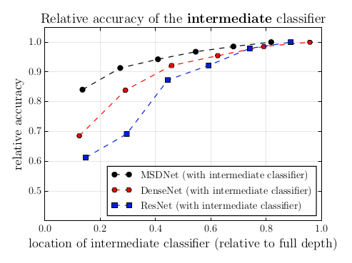
It hurts. Pretty badly. DenseNets are once again less sensitive to this effect, but the performance of the intermediate classifier is still unsatisfying.
Solution/Mitigation: Multi-scale feature maps
To mitigate this harmful effect, the authors suggest maintaining feature maps of multiple scales at all layers. This is pretty annoying to describe with words, so let’s jump into the architecture to see how it is implemented.
The architecture
As expected, the resulting design combines dense connections with multi-scale feature maps to yield the architecture of the Multi-Scale DenseNet, taking the following form:

The MSDNet architecture. Each layer maintains feature maps at multiple scales, enabling early classifiers to operate on coarse-level features. The feature maps at a given scale and layer are the concatenation of two elements: the result (in blue) of strided convolution on the finer-scale features from the previous layer, and the result (in red) of regular convolution on the same scale features from multiple previous layers via dense connections.
This is not your typical CNN architecture, so let’s break it down bit by bit: first the layers and the connections, then the classifiers and their repartition, and finally the training details and the loss function.
Layers
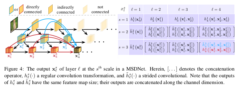
As described in the figures, the model is structured as a 2-dimensional grid $S \times L$, with $L$ the number of layers (analogous to the depth in standard networks) and $S$ the number of scales at each layer.
The first layer $l=1$ is quite unique, since it “seeds” all scales $s = 1, …, S$ of the feature maps. The finer scale $s=1$ is the result of a regular convolution $h$ on the original image. For subsequent scales, the feature map at scale $s+1$ is the result of strided convolution $\tilde{h}$ (which is just really regular convolution with a stride of at least 2) to the features at scale $s$. Given that strided convolution results in downsampling of the input (like max pooling), the feature map at scale $s+1$ is smaller than the one at scale $s$. This enables coarser-level, global information to be encoded already in the first layer.
The next layers maintain all scales that were previously seeded. The output of layer $l$ at scale $s$ is the concatenation of two elements:
- The result of regular convolution $h$ on all previous feature maps (dense connection) at scale $s$ from layers $l’=1, …, l-1$ (in red).
- The result of strided convolution $\tilde{h}$ on all previous feature maps (dense connection) at scale $s-1$ from layers $l’=1, …, l-1$ (in blue, performing the downsampling of finer-scale features that is common in CNNs).
Classifiers
Following the same principle of dense connections, the classifiers take as input the concatenation of all coarse feature maps from all previous layers. In practice they are only attached to some intermediate layers, and their behavior depends on the task at hand:
- In anytime prediction, the classifiers are evaluated sequentially until the budget is exhausted, and only the last prediction is output.
- In budgeted batch classification, for each test example, the classifiers are evaluated sequentially until a sufficient level of confidence in prediction is found. However, determining the “sufficient level” part can be quite tricky, since you have to distribute a budget across multiple samples without knowing the difficulty of each. You cannot afford to fully evaluate the network on each one, yet you have to be confident enough in your prediction, while not knowing how long it is going to take for individual examples to reach this level of confidence. The authors therefore rely on a probabilistic model of the difficulty of the inputs to design the optimal threshold that wll determine whether or not we stop running a given input through the network.
Training details
We now have a network with multiple classifiers that need to be trained jointly. To do so, we unsurprisingly use cross-entropy $L(f_k)$ for all classifiers $f_k$, but we still need to combine those losses to perform joint optimization. The most natural solution is to take a weighted sum of all the individual losses, such as the final loss of the model is:
[L(f) = \sum_k w_k L(f_k)]
If the budget distribution $P(B)$ is known, we can use the weights to incorporate prior knowledge about the budget $B$ in the learning. Empirically, we find that using uniform weights $\forall k, w_k=1$ works well in practice.
A glance at the results
Now that we’ve gone so far, let’s just check that MSDNet performs well on the tasks it’s been designed to solve, namely anytime prediction and budgeted batch classification.
Anytime prediction
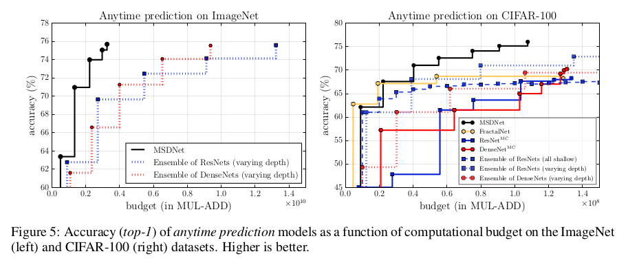
In anytime prediction, for each test example, the model is run until an unknown budget $B$ is exhausted, and is forced to output its latest prediction. As discussed earlier, typical baselines to compare against are ensembles of CNNs, here ensembles of ResNets and ensemble of DenseNets, that are evaluated sequentially until the budget is exhausted. Other baselines include deeply supervised networks (here ResNetMC and DenseNetMC) and FractalNet. Going into details of these models is beyond the scope of this article; check the original papers to read about these interesting architectures.
MSDNet shows excellent performance compared to all other baselines across all budgets, except FractalNet in low budget, where the performances are comparable. Note that, in extremely low budgets, the ensembles have a significant advantage since the first network (the only one evaluated) is directly optimized for prediction; yet MSDNet performance remains very satisfying. The limitations of ensembles appear very quickly when the budget increases, since they waste a lot of computation.
Budgeted batch classification
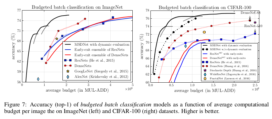
In budgeted batch classification, the model is granted a finite known computational budget $B$ to classify a set of examples, and can spend it freely across examples. This encourages the use of dynamic evaluation, where easy examples are exited early while hard examples are run throughout the network until a sufficient level of confidence in classification is reached. The baselines are similar to the previous ones.
Three MSDNets are trained with different depths, in order to cover a wide range of computational budgets, and the chosen model is selected depending on the budget, based on validation performance; this explains the three black curves. Once again, MSDNet prove very performant across all budgets, outperforming all baselines by a wide margin. In particular, MSDNet perform much better than deeply supervised networks, highlighting the importance of coarse-level features for classification at early stages.
Bonus points - Visualization
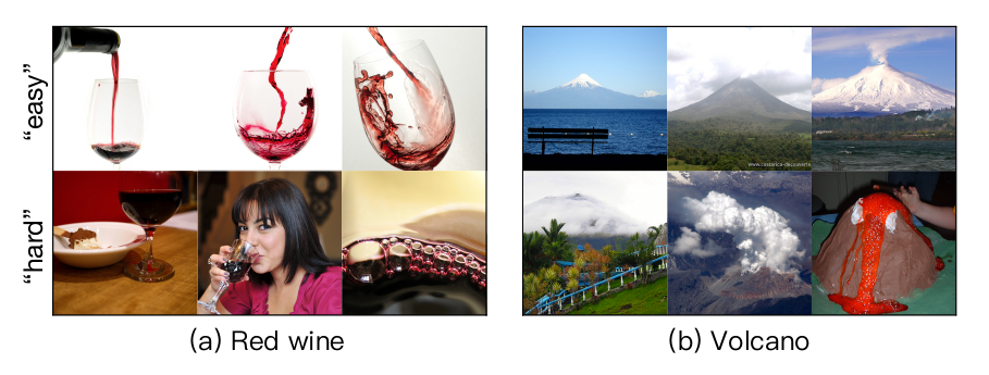
Samples from ImageNet classes red wine and volcano. Thanks to the dynamic evaluation, “easy” examples are early-exited while “hard” examples are run through larger parts of the network.
To assess the relevance of dynamic evaluation and the calibration of confidence of the classifiers, it is interesting to examine which examples are early exited, and which ones are run through the entire network. As the figure above suggests, MSDNet seem able to quickly classify typical class examples, while non-typical images are granted a larger budget.